Visual Recognition for Vietnamese Foods
Imagine that you are a world traveller and are traveling to a country famous for its street foods. Walking in a night market street full of food trucks with many delicious-looking options, you have no idea what these foods are and whether they contain any ingredient you are allergic to. You want to ask the local but you don’t know the language. You wish that you have an app on your phone that allows you to take a picture of that food you want to have and will return all the information you need to know about it.
It’s one simple application of computer vision that can make our life better, besides many other applications being implemented in autonomous driving or cancer detection.
Today we are going to build a world-class image classifier using the fastai library to classify 11 popular Vietnamese dishes. The fastai library is built on top of PyTorch and allows us to quickly and easily build the latest neural networks and train our models to receive state-of-the-art results.
Before we begin, let’s load packages that we are going to use in this project.
%reload_ext autoreload
%autoreload 2
%matplotlib inline
import os
import numpy as np
import urllib.request
from fastai.vision import *
from fastai.metrics import error_rate
from PIL import Image, ImageFile
ImageFile.LOAD_TRUNCATED_IMAGES = True
Looking at the data
I have built an image dataset of popular Vietnamese dishes using the Bing Image Search API by following PyImageSearch’s tutorial. We can directly download this dataset from Google Drive.
%%time
# Download and unzip
if not os.path.exists("data"):
    !wget -O "dataset.zip" "https://www.googleapis.com/drive/v3/files/13GD8pcwHJPiAPbPtm6KeC20Qw1zm9xdy?alt=media&key=AIzaSyCmo6sAQ37OK8DK4wnT94PoLx5lx-7VTDE"
    !unzip dataset.zip
    !rm dataset.zip
Each class is stored in a seperate folder in data and we can use ImageDataBunch.from_folder to quickly load our dataset. In addition, we resize our images to 224 x 224 pixel and use get_transforms to flip, rotate, zoom, warp, adjust lighting our original images (which is called data augmentation, a strategy that enables practitioners to significantly increase the diversity of data available for training models, without actually collecting new data). We also normalize the images using statistics from ImageNet dataset.
path = Path("./data/")
np.random.seed(42)
data = ImageDataBunch.from_folder(path, train='.', ds_tfms=get_transforms(),
                                  valid_pct=0.2, bs=64, size=224).normalize(imagenet_stats)
The dataset has more than 6k images and we use 20% of them as a validation set.
len(data.train_ds), len(data.valid_ds)
(4959, 1239)
Let’s look at some samples:
data.show_batch(rows=3, figsize=(7, 6))
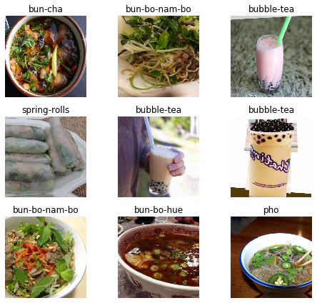
The dataset has a total of 11 classes. They are:
print("Number of classes: ", len(data.classes))
print("Classes: ", data.classes)
Number of classes:  11
Classes:  ['banh-mi', 'banh-xeo', 'bubble-tea', 'bun-bo-hue', 'bun-bo-nam-bo', 'bun-cha', 'bun-dau-mam-tom', 'che', 'hu-tieu', 'pho', 'spring-rolls']
Training: ResNet-50
Now we will finetune a ResNet-50 model on our customized dataset. ResNet is from the paper Deep Residual Learning for Image Recognition and is the best default model for computer vision. This ResNet-34 model is trained on ImageNet with 1000 classes, so first we need to initialize a new head for the model to be adapted to the number of classes in our dataset. The cnn_learner method will do this for us (Read documentation).
Then we will train the model in two stages:
- first we freeze the body weights and only train the head,
- then we unfreeze the layers of the backbone and fine-tune the whole model.
Stage 1: Finetune the top layers only
learn = cnn_learner(data, models.resnet50, metrics=error_rate, pretrained=True)
We will train the model for 20 epoches following the 1cycle policy. The number of epoches we need to train depends on how different the dataset is from ImageNet. Basically, we train the model until the validation loss stops decrease. The default learning rate here is 3e-3.
learn.fit_one_cycle(20)
| epoch | train_loss | valid_loss | error_rate | time |
|---|---|---|---|---|
| 0 | 1.356109 | 0.657256 | 0.206618 | 01:31 |
| 1 | 0.870719 | 0.560793 | 0.167070 | 01:27 |
| 2 | 0.687549 | 0.526645 | 0.167877 | 01:32 |
| 3 | 0.621711 | 0.444908 | 0.143664 | 01:27 |
| 4 | 0.493342 | 0.397156 | 0.126715 | 01:28 |
| 5 | 0.435479 | 0.381771 | 0.123487 | 01:27 |
| 6 | 0.373893 | 0.389900 | 0.121065 | 01:28 |
| 7 | 0.325564 | 0.371386 | 0.112994 | 01:28 |
| 8 | 0.295842 | 0.349679 | 0.106538 | 01:29 |
| 9 | 0.271255 | 0.348150 | 0.098467 | 01:28 |
| 10 | 0.233799 | 0.317944 | 0.091203 | 01:28 |
| 11 | 0.205257 | 0.306772 | 0.086360 | 01:27 |
| 12 | 0.171645 | 0.310830 | 0.084746 | 01:28 |
| 13 | 0.159442 | 0.293081 | 0.078289 | 01:27 |
| 14 | 0.137362 | 0.295972 | 0.083939 | 01:29 |
| 15 | 0.112108 | 0.289382 | 0.084746 | 01:26 |
| 16 | 0.093431 | 0.279121 | 0.083939 | 01:30 |
| 17 | 0.094814 | 0.281516 | 0.079903 | 01:29 |
| 18 | 0.083980 | 0.277226 | 0.073446 | 01:33 |
| 19 | 0.090189 | 0.274643 | 0.081517 | 01:28 |
learn.save('resnes50-stage-1')
Stage 2: Unfreeze and finetune the entire networks
At this stage we will unfreeze the whole model and finetune it with smaller learning rates. The code below will help us find the learning rate for this stage.
learn.load('resnes50-stage-1')
learn.lr_find()
learn.recorder.plot()
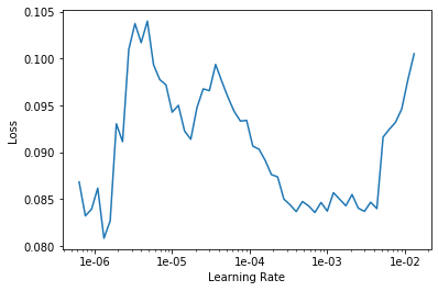
When finetuning the model at state 2, we will use different learning rates for different layers. The top layers will be update at greater rates than the bottom layers. As a rule of thumb, we use learning rates between (a, b), in which:
- a is taken from the LR Finder above where the loss starts to decrease for a while,
- b is 5 to 10 times smaller than the default rate we used in stage 1.
In this case, the learning rate we will use is from 3e-6 to 3e-4 We continnue to train the model until the validation loss stops decreasing.
learn.unfreeze()
learn.fit_one_cycle(8, max_lr=slice(3e-6, 3e-4))
| epoch | train_loss | valid_loss | error_rate | time |
|---|---|---|---|---|
| 0 | 0.077156 | 0.277789 | 0.079903 | 01:30 |
| 1 | 0.089096 | 0.269736 | 0.075061 | 01:30 |
| 2 | 0.092252 | 0.282279 | 0.079096 | 01:29 |
| 3 | 0.074603 | 0.265167 | 0.067797 | 01:31 |
| 4 | 0.071408 | 0.278237 | 0.074253 | 01:33 |
| 5 | 0.047503 | 0.250248 | 0.065375 | 01:29 |
| 6 | 0.037788 | 0.249852 | 0.070218 | 01:30 |
| 7 | 0.035603 | 0.251429 | 0.066990 | 01:29 |
After two stages, the error rate on the validation set is about 6% and the accuracy for our dataset with 11 classes is 94%. That’s a pretty accurate model. It’s a good practice to save the current stage of the model in case we want to train it for more epoches.
learn.save('resnes50-stage-2')
Evaluation
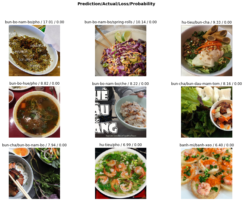
Now let’s look on the model’s predictions. Specifically, we will look at examples where the model makes wrong predictions. Below are 9 examples with the top losses, meaning on these examples the model gives the actual class a very low score.
learn.load('resnes50-stage-2')
interp = ClassificationInterpretation.from_learner(learn)
losses, idxs = interp.top_losses()
interp.plot_top_losses(9, figsize=(15,11))
The confusion matrix below will us a big picture of which pair of dishes make our model confused. The number of wrong predictions are quite low.
interp.plot_confusion_matrix(figsize=(12,12), dpi=60)
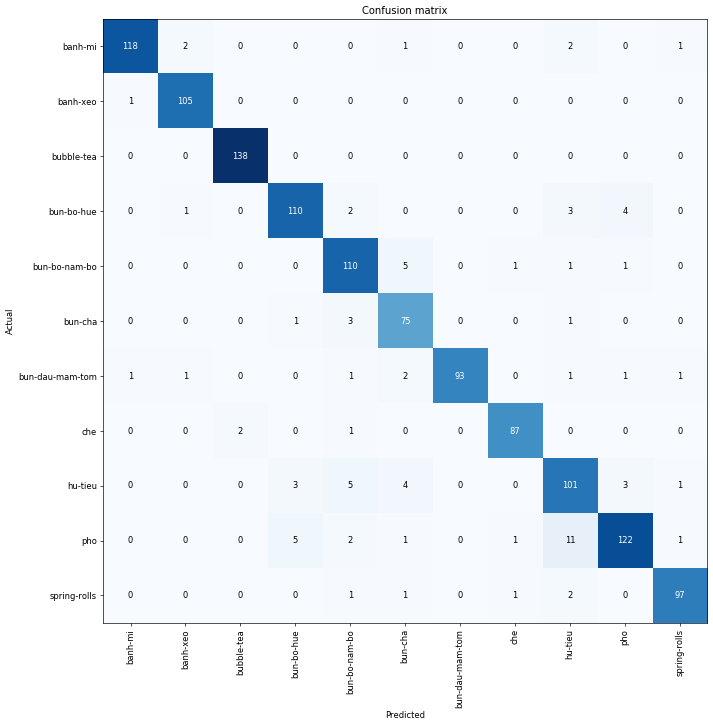
interp.most_confused(min_val=3)
[('pho', 'hu-tieu', 11),
 ('bun-bo-nam-bo', 'bun-cha', 5),
 ('hu-tieu', 'bun-bo-nam-bo', 5),
 ('pho', 'bun-bo-hue', 5),
 ('bun-bo-hue', 'pho', 4),
 ('hu-tieu', 'bun-cha', 4),
 ('bun-bo-hue', 'hu-tieu', 3),
 ('bun-cha', 'bun-bo-nam-bo', 3),
 ('hu-tieu', 'bun-bo-hue', 3),
 ('hu-tieu', 'pho', 3)]
Production
After being satisfied with our model, we can save it to disk and use it to classify new data. We can also deploy it into a magical app that I described at the beginning of the notebook.
# Export model
learn.export()
For inference, we also want to run the model on CPU instead of GPU.
defaults.device = torch.device('cpu')
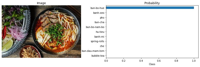
The functions below will download an image from an URL and use the model to make prediction for that image.
def open_image_url(url):
    """Download image from URL, return fastai image and PIL image."""
    urllib.request.urlretrieve(url, "./img/test.jpg")
    return open_image("./img/test.jpg"), Image.open("./img/test.jpg")

def predict(url):
    """Make prediction for image from url, show image and predicted probability."""
    img, pil_img = open_image_url(url)
    pred_class, pred_idx, outputs = learn.predict(img)
    print("Predicted Class: ", pred_class)
    print(f"Probability: {outputs[pred_idx].numpy() * 100:.2f}%")

    plt.figure(figsize=(15, 4))
    # Show image
    plt.subplot(1, 2, 1)
    plt.imshow(pil_img)
    plt.axis('off')
    plt.title('Image')

    # Plot Probabilities
    plt.subplot(1, 2, 2)
    pd.Series(outputs, data.classes).sort_values().plot(kind='barh')
    plt.xlabel("Class")
    plt.title("Probability");
# Load model
learn = load_learner(path)
# Make prediction from URL
url = str(input("URL: "))
predict(url)
URL:  https://i.pinimg.com/originals/9b/63/d7/9b63d76a44be020e03eeaec0a1134e95.jpg


Predicted Class:  bun-bo-hue
Probability: 99.99%
I have also built a web app for this model. Check it out below:

Conclusion
We have walked through the whole pipeline to finetune a ResNet-50 model on our customized dataset, evaluate its strengths and weaknesses and deploy the model for production. With the fastai library, we can quickly achieve state-of-the-art results with very neat and clean codes.
In this project, we built a classifier for only 11 popular Vietnamese dishes, but we can easily scale up the model by collecting more data for hundreds or thounsands of classes following this PyImageSearch’s tutorial.
I have seen many interesting ideas using computer vision, such as Plantix, a plant doctor app which can tell what diseases your plants might have from a single photo and how you should take care of them. And yes, with some software engineering skills, some data and an idea, you can build your own impactful computer vision application. I look forwards to seeing these applications make the world a better place in all directions.


Leave a comment